Feed-forward neural doodle
Sometimes you sigh you cannot draw, aren’t you? It takes time to master the skills, and you have more important things to do :) What if you could only sketch the picture like a 3-years old and everything else is done by a computer so your sketch looks like a real painting? It will certainly happen in near future. In fact several algorithms that do the thing very well were proposed recently, yet they take at least several minutes to render your masterpiece using a high-end hardware. We make a step towards making such things available for everybody and present an online demo of our fast algorithm.
The following text describes the way it is done. The code is available on github. The project is closely related to our ICML 2016 paper:
D. Ulyanov, V. Lebedev, A. Vedaldi, and V. Lempitsky. Texture networks: Feed-forward synthesis of textures and stylized images. In International Conference on Machine Learning (ICML), 2016. [paper|bibtex]
Background
Artistic style
A year ago a groundbreaking paper [Texture Synthesis Using Convolutional Neural Networks, Gatys et al., NIPS’15] which followed by an amazing extension [A Neural Algorithm of Artistic Style, Gatys et al.] was published. They proposed a way to generate textures and transfer style (synonym for texture) from one image onto another.
Texture generation and stylization were achieved mainly by defining a function $L_{style}(x;y)$, which describes whether an input image $x$ have the same style (texture) as the given style image $y$. Important, that $L_{style}(x;y)$ is differentiable, which means new images with given style can be generated by optimization! Just run your favorite optimizer to minimize $L_{style}(x;y)$ with respect to target image $x$ starting from a random image. The results turn out to be very cool, yet the optimization requires high-end hardware and time.
The way loss $L_{style}(x;y)$ is defined is the following. First, we need a convolutional neural network pretrained for object recognition, e.g. VGG-19. Fix a set of layers ${l}$ and consider the activations $F^l(x) \in R^{C_l \times M_l N_l}$ at layer $l$ observed when image $x$ fed into the network. Here $C_l$ is a number of filters, $M_l$, $N_l$ – spatial dimensionalities. Now the feature correlations are computed:
\[G_{ij}^l(x) = \sum_{k=1}^{M_l N_l} F_{ik}^l(x) F_{jk}^l(x)\]and the style loss is defined as following:
\[L_{style}(x;y) = \sum_l \frac{1}{M_l N_l} \sum_{ij} (G_{ij}^l(x) - G_{ij}^l(y)).\]You may notice, that $\frac{1}{M_lN_l}G^l$ is an empirical covariance matrix for a dataset of $M^l N^l$ “pixels” at the level $l$, where each “pixel” has exactly $C_l$ features. This means we fit a Gaussian distribution with zero mean to the pixels of the target image $x$ and will optimize pixels in such a way, that fitted pixel distribution is similar to the distribution of pixels for the style image $y$. In fact, consider a true distribution $P$ and model distribution $Q \sim \mathcal{N}(0, \Sigma)$. Let’s solve $\Sigma^* = \arg \min_{\Sigma} KL(P||Q)$. Setting derivatives to zero it is easy to find, that \(\Sigma^* = \mathbb{E}_{x \sim P} x^Tx\) for any $P$. Since we do not have access to true distribution $P$ and always fit $Q$ to the data, we substitute the last equation with an empirical variant, which is exactly $ \frac{1}{M_l N_l} G(x^* ) = \frac{1}{M_l N_l} G(y)$ and $x^{*} = \arg \min_x L_{style}(x;y)$.
One more note: the paper actually suggests $\frac{1}{4 M_l^2 N_l^2}$ normalization but I found every implementation on github uses slightly different constants. Setting the factor to $\frac{1}{M_l N_l}$ lets you explain everything with distributions.
Style transfer requires one more loss called content loss which makes sure the resulting image does not differ too much from a given image. You can find the details in the paper.
Making artistic style faster: Texture networks
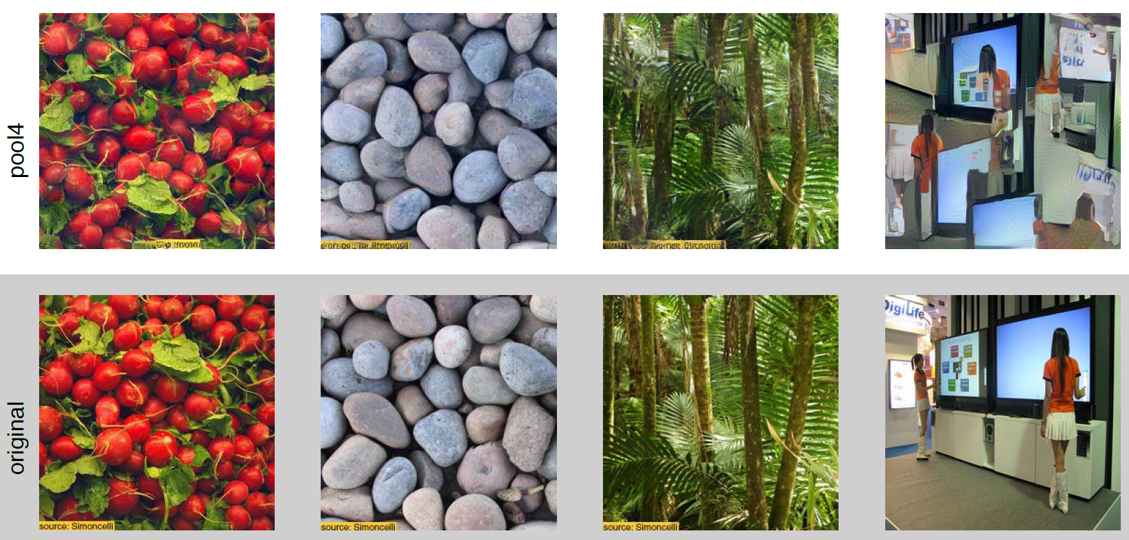
In our paper [Texture Networks: Feed-forward Synthesis of Textures and Stylized Images, Ulyanov et. al., ICML’16] we describe the way to archive at least $500\times$ faster texture generation and stylization. The idea is to map a random noise $z \sim \text{uniform}(0,1)$ onto a manifold $X$, which consists of images with low style loss $L_{style}(x;y)$ ($y$ is style image). The mapping can be done by a neural network $g_{\theta}(z)$ and all we need to do is to learn its parameters! This is straightforward, just think of $L_{style}$ as of $L_2$ (MSE) loss or any other loss function, which compares instances in an object space.
To learn a network generate textures we sample a batch of tensors, filled with random numbers. The generator processes these tensors and produces a batch of images $x = g_{\theta}(z)$. The images $x$ are scored with $L_{style}(x;y)$ and gradient $\frac {\partial L_{style}(x;y)}{\partial x}$ is computed. This gradient gets backpropagated into the network $g_{\theta}(z)$ and the parameters $\theta$ updated accordingly. The process is repeated for several thousands iterations. Now to generate a new texture sample you only need to sample $z$ and do a single forward pass with a network.
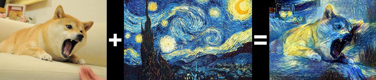
The stylization is done in the similar way, but now we show the generator the image it needs to stylize along with the noise $z$.
The code is available on github.
Patch-based artistic style
A competing approach to the original distribution matching idea of artistic style is a patch-based approach described in the paper by Chuan Li and Michael Wand. They generate an image $x$ in such a way, that every pixel at each layer $l$ of neural network has a similar one in the style image. This can yield awesome results when there is no need to preserve the distribution.
Neural doodles
Two month ago Alex Champandard created neural doodles on top of the patch-based method for artistic style. The idea is to rerender an image manipulating its semantic maps. After that I approached neural doodles with distribution matching variant. My implementation produced nice results and turned out to be faster than Alex’s version since patch manipulations are computationally expensive, which was the reason to call it “fast-neural-doodle”.
My “fast-neural-doodle” is, in fact, nothing more than a version of original artistic style algorithm with masks, or semantic map. The semantic map splits the image $x$ into $R$ semantic regions ${R_i}(x)$. We actually want to learn style of each region and transfer it to corresponding region in the target semantic mask. We already know how to transfer style, but we should be careful with the normalization constants. Now, for each region $r = 1,2,\dots, R$ at layer $l$ let $F^{l,r}(x) = F^{l}(x) \circ R^{l,r}(x)$ ($\circ$ stands for element-wise multiplication) and compute gram matrices $G^{l,r}$:
\[G_{ij}^{l,r}(x) = \sum_k F_{ij}^{l,r}(x) F_{jk}^{l,r}(x)\]Now, when defining the loss we need to normalize each $G^{l,r}(x)$ by the number of pixels in a region $R^{l,r}(x)$, which is the area of mask $R_{l,r}(x)$. Dividing the area by the total number of pixels (constant for each layer $l$) we get an appropriate normalization:
\[C^{l,r}(x) = \frac{1}{M_l N_l} \sum_{ij} R_{ij}^{l,r}(x)\]If you still can remember the meaning of each index the final formula should be easy. In fact, again, we are just matching empirical covariance matrices.
\[L_{style}(x;y) = \sum_l \sum_r \sum_{ij} (C^{l,r}(x) G_{ij}^l(x) - C^{l,r}(y) G_{ij}^l(y)).\]Following the artistic style paper we use conv1_1,conv2_1,conv3_1,conv4_1,conv5_1 layers of VGG-19 and L-BFGS optimizer. You can find the code here.
Online (feed-forward) neural doodles
Finally, we have a way to make artistic style faster, we can apply it to neural doodles, but we need to think how to incorporate masks into the learning process. First we need to generate a masks dataset.
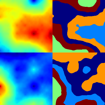
The only way to generate random (but smooth) masks I could make up was to make use of height-maps generators. It was not that simple to find a good implementation, but finally github.com/buckinha/DiamondSquare was used. It implements diamond-square algorithm and written in python.
Now when we can generate smooth surfaces, let’s cluster the pixels by applying K-means. To make sure the segmentation is not too ragged and does not have too small regions we filter the mask with median filter. The next picture shows a height-map and a resulting mask.
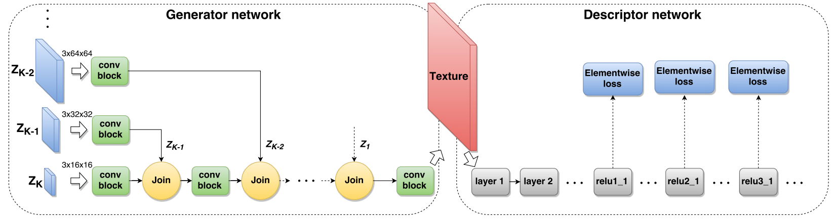
We are all set up to start learning process. The input is formed by concatenation of mask (of size num_regions x W x H with zeros and ones) and a noise tensor of similar size. Network $g$ produces an image, which scored next with the $L_{style}$ described above.
It is interesting how we define masks $R^{l,r}$ at a layer $l$. The obvious way is to scale the mask to match spatial dimensions of activations $F^l$ with a standard nearest-neighbor or bilinear interpolation. In fact the deeper you go inside neural net, the less clear the border between regions become. After two 3x3 convolutions each pixel aggregates information from 5x5 patches and now for some pixels you cannot certainly say what region they belong to. This motivates to blur the mask accordingly to receptive field of corresponding layer in VGG as we go through. Use 3x3 mean filter for mask when the data goes through convolutions and average pooling along with pooling layers.
Notes
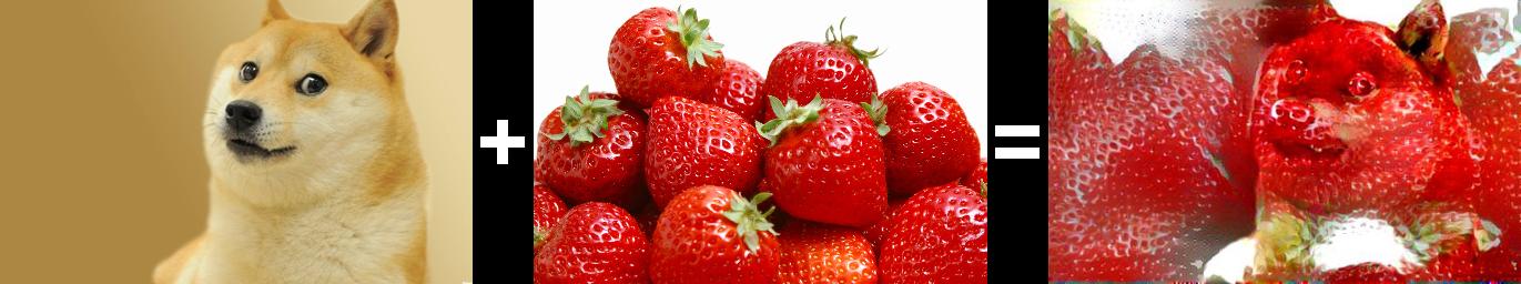
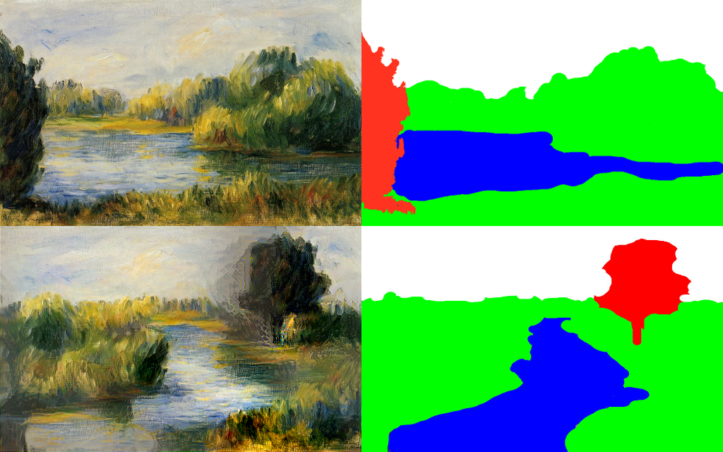
- If we set the seed and try different masks, we’ll see the network learned to produce a full-resolution image for each semantic style and then multiply it by mask. Hard to say what exactly we expected, but generator tends to strictly follow the edges between the regions.
- Some padding-related problems are very annoying and result in horizontal lines. Look at the example above.
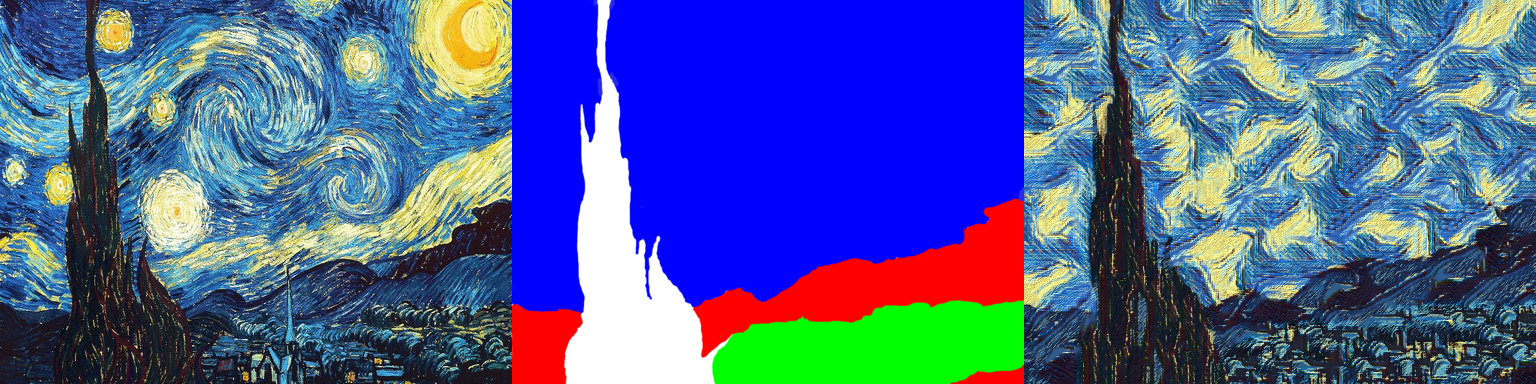
- The training procedure is weak in a way. Assume a huge region with a lot of variety (sky in starry night). The masks we generate can have almost zero area for this region, still we want distributions to be preserved.
- It was fun.
All links in one place
- Artistic style
- Texture networks
- fast-neural-doodle
- Feed-forward neural doodle
- Alex is working on a fast version of his patch-based approach. Check out his repo.