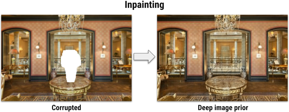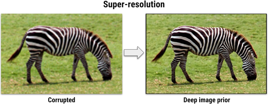
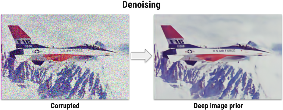
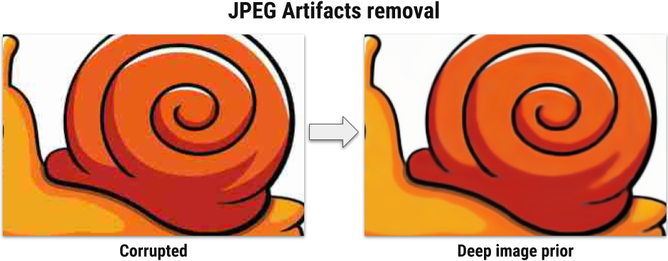
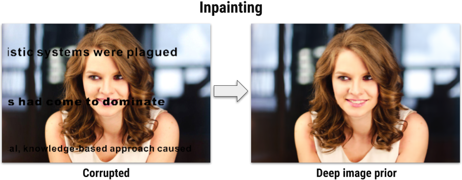
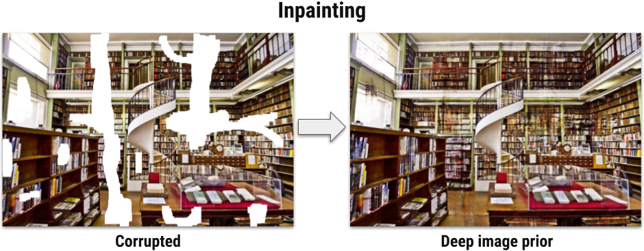
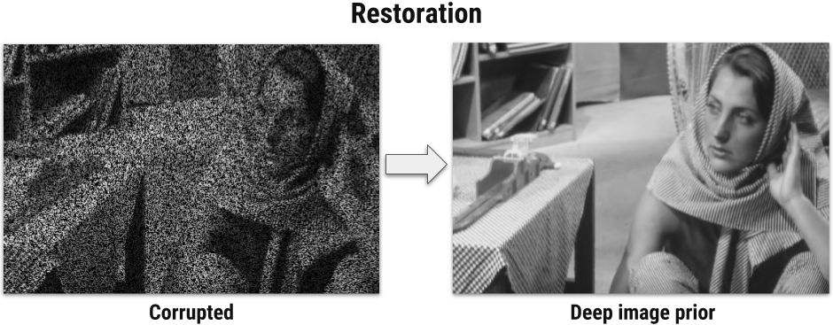
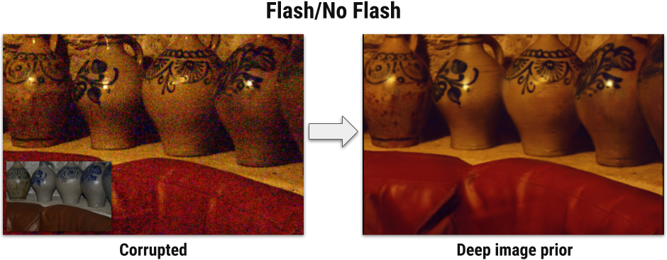
Deep convolutional networks have become a popular tool for image generation and restoration. Generally, their excellent performance is imputed to their ability to learn realistic image priors from a large number of example images. In this paper, we show that, on the contrary, the structure of a generator network is sufficient to capture a great deal of low-level image statistics prior to any learning. In order to do so, we show that a randomly-initialized neural network can be used as a handcrafted prior with excellent results in standard inverse problems such as denoising, super-resolution, and inpainting. Furthermore, the same prior can be used to invert deep neural representations to diagnose them, and to restore images based on flash-no flash input pairs.
Apart from its diverse applications, our approach highlights the inductive bias captured by standard generator network architectures. It also bridges the gap between two very popular families of image restoration methods: learning-based methods using deep convolutional networks and learning-free methods based on handcrafted image priors such as self-similarity.


In image restoration problems the goal is to recover original image $x$ having a corrupted image $x_0$. Such problems are often formulated as an optimization task: \begin{equation}\label{eq1} \min_x E(x; x_0) + R(x)\,, \end{equation} where $E(x; x_0)$ is a data term and $R(x)$ is an image prior. The data term $E(x; x_0)$ is usually easy to design for a wide range of problems, such as super-resolution, denoising, inpainting, while image prior $R(x)$ is a challenging one. Today's trend is to capture the prior $R(x)$ with a ConvNet by training it using large number of examples.
We first notice, that for a surjective $g: \theta \mapsto x$ the following procedure in theory is equivalent to \eqref{eq1}: $$\min_\theta E(g(\theta); x_0) + R(g(\theta)) \,.$$ In practice $g$ dramatically changes how the image space is searched by an optimization method. Furthermore, by selecting a "good" (possibly injective) mapping $g$, we could get rid of the prior term. We define $g(\theta)$ as $f_\theta(z)$, where $f$ is a deep ConvNet with parameters $\theta$ and $z$ is a fixed input, leading to the formulation $$\min_\theta E(f_\theta (z); x_0) \,.$$ Here, the network $f_\theta$ is initialized randomly and input $z$ is filled with noise and fixed.
In other words, instead of searching for the answer in the image space we now search for it in the space of neural network's parameters. We emphasize that we never use a pretrained network or an image database. Only corrupted image $x_0$ is used in the restoration process.
See paper and supplementary material for details.
Click on the image below and use left and right arrows or swipe.